Ultrasound Physics for Beginners: 10 Principles for Better POCUS

Ultrasound physics becomes practical when it changes what you do with the probe. The image is not a photograph of anatomy. It is a map built from returning echoes, timing assumptions, signal processing, and the settings you choose. Understanding ten relationships—frequency, penetration, pulse-echo timing, impedance, angle, attenuation, echogenicity, controls, artifacts, and Doppler—helps you select the right transducer, improve the view, and recognize when the screen may be misleading.

This guide focuses on ultrasound physics for beginners: the concepts most useful at the bedside, not every formula taught on a sonography physics examination. The ACEP SonoGuide physics chapter and the StatPearls review of ultrasound physics and instrumentation provide additional technical depth.

1. Frequency and wavelength move in opposite directions.
2. Higher frequency improves detail but reduces penetration.
3. Pulse-echo timing creates image depth.
4. Acoustic impedance differences create echoes.
5. Angle changes how much sound returns to the probe.
6. Attenuation weakens the beam with depth.
7. Echogenicity describes relative brightness.
8. Gain, depth, focus, and presets optimize the display and beam.
9. Artifacts can reveal pathology or imitate it.
10. Doppler estimates motion from frequency shift.

Before the 10 principles: how the transducer builds an image

Most conventional ultrasound transducers use piezoelectric elements. A brief electrical signal makes the elements change shape and vibrate, converting electrical energy into a mechanical pressure wave. The probe then listens: returning echoes deform the elements and are converted back into electrical signals for processing. Some newer systems use micromachined transducer technology instead, but the same transmit–listen sequence still applies.

Resolution describes whether the system can display two nearby reflectors as separate structures. Axial resolution applies to reflectors lying one behind the other along the beam and improves with a shorter spatial pulse length. Lateral resolution applies to reflectors lying side by side and depends largely on beam width, so it is usually best near the focal zone. Practically, use the highest frequency that still penetrates to the target and place the focus at or just deeper than the region of interest; those choices improve different dimensions of detail.

Two kinds of spatial resolution: shorter spatial pulse length improves separation along the beam (axial resolution). A narrower beam improves separation across it (lateral resolution). These are different properties; increasing gain does not improve either one.

1. Frequency and wavelength move in opposite directions

Frequency is the number of wave cycles that pass a point each second. Diagnostic ultrasound operates at frequencies far above human hearing and usually displays transducer frequency in megahertz (MHz), or millions of cycles per second. Wavelength is the physical length of one cycle.

Within a given medium, propagation speed is approximately fixed, so frequency and wavelength have an inverse relationship: as frequency rises, wavelength becomes shorter. Shorter wavelengths can distinguish smaller structures along the beam more effectively. That is one reason higher-frequency imaging can provide finer spatial detail.

Practical consequence: frequency is not a “quality” control that should always be maximized. It is a tradeoff. The correct frequency is the highest one that still reaches the target and returns useful echoes.

2. Higher frequency improves resolution but reduces penetration

Higher-frequency waves are attenuated more rapidly as they travel through tissue. They can create excellent detail near the transducer but may not return enough signal from a deep target. Lower-frequency waves generally penetrate farther, although the image contains less fine detail.

This relationship explains why transducers are matched to the acoustic window and target depth. Frequency ranges overlap, and modern devices may use broad bandwidths or multipurpose transducer technology, so the table below describes common patterns rather than absolute rules.

Transducer pattern	Physics advantage	Common POCUS uses	Common limitation
Linear	Typically higher frequency and strong near-field detail	Vessels, soft tissue, pleura, musculoskeletal structures, superficial procedures	Limited penetration and a rectangular footprint that may not fit every window
Curvilinear	Typically lower frequency with a broad deep field of view	Abdomen, pelvis, eFAST, renal and bladder imaging	Less superficial detail than a high-frequency linear transducer
Phased array	Small footprint and lower-frequency penetration between ribs	Focused cardiac, thoracic, and selected abdominal views	Narrow near field and less detail for very superficial targets

Beginner check: if the target is deep and disappearing, consider a lower-frequency transducer or frequency setting before simply increasing gain. If a superficial target looks coarse, consider a higher-frequency option and reduce the displayed depth.

Recorded app example · Essentials

Choose a probe, then check the explanation

This short practice question connects target depth with probe selection. Watch the answer and the app’s rationale, then return to the frequency–penetration trade-off above.

Read the clip description

The question asks which transducer is best for superficial structures such as vessels and tendons. The linear-transducer answer is selected. The app marks it correct and explains the value of high-frequency imaging for superficial detail.

Explore the app

3. Pulse-echo timing creates image depth

The transducer sends a short pulse, then listens for returning echoes. The system estimates how deep a reflector is by measuring the round-trip travel time. Because the pulse travels to the reflector and back, the distance calculation uses one-half of the total travel path.

Clinical scanners assume an average speed of sound in soft tissue of approximately 1,540 meters per second. The assumption is useful, but the body is not a uniform block of soft tissue. Sound travels at different speeds in fat, fluid, bone, and other materials. When reality differs from the machine’s assumptions, structures may be misplaced, duplicated, or distorted.

The same timing principle explains why increasing depth can reduce frame rate. The machine must wait longer for echoes to return from the bottom of the image before sending the next pulse. Using substantially more depth than necessary can therefore make a moving image feel less responsive and makes the target occupy less of the screen.

Practical consequence: set depth so the target and the anatomy immediately beyond it are visible. Do not crop away essential context, but do not spend most of the screen imaging tissue that is irrelevant to the focused question.

4. Acoustic impedance differences create echoes

Acoustic impedance describes a material’s resistance to sound propagation and depends on its density and the speed of sound within it. When a wave reaches a boundary between tissues with different acoustic impedances, some energy is reflected and some continues deeper.

A larger impedance mismatch generally produces a stronger reflection. Boundaries between similar soft tissues return weaker echoes. Boundaries involving air or bone produce large mismatches, which is why air and cortical bone can prevent visualization of deeper anatomy.

Ultrasound gel is not cosmetic. It removes the thin layer of air that would otherwise sit between the probe and skin. Better coupling allows acoustic energy to enter the body and returning echoes to reach the transducer.

Practical consequence: when an image suddenly disappears, check contact before changing multiple settings. Add gel, stabilize the footprint, reposition around bowel gas or ribs, and look for a different acoustic window.

5. Angle changes the returning signal

Many smooth tissue boundaries behave like mirrors. When the beam strikes a specular reflector close to perpendicular, more sound returns toward the transducer and the interface appears brighter. When the beam strikes at an oblique angle, reflected energy may travel away from the probe, making the same structure appear faint or absent.

This is why a few degrees of tilt, rock, or heel-toe movement can transform an image. The anatomy has not changed; the insonation angle has. Tendons, ligaments, nerves, and some muscle interfaces can be particularly angle dependent. The resulting change in brightness is called anisotropy and can imitate abnormality if the operator does not test another angle.

Refraction is different. A beam can bend as it crosses a boundary where propagation speed changes. The machine assumes a straight path, so refracted echoes may be displayed in the wrong location or create edge shadows and duplicated structures.

• If a linear structure becomes unexpectedly dark: make a small angle correction before declaring it abnormal.
• If anatomy seems duplicated or displaced: scan from another window and consider refraction or mirror artifact.
• If a view is almost correct: change one movement at a time—slide, rotate, tilt/fan, rock, or compress—then observe the result.

6. Attenuation weakens the beam with depth

Attenuation is the progressive loss of ultrasound energy as the wave travels. Absorption converts some acoustic energy to heat; reflection and scattering redirect other portions of the beam. Attenuation increases with distance and, in soft tissue, generally increases with frequency.

The machine must compensate for the weaker echoes returning from deeper tissue. Overall gain amplifies received signals across the image. Time-gain compensation (TGC) changes amplification by depth, allowing the operator to brighten a deep region without equally brightening the near field.

Attenuation also creates useful clues. A calcified structure or bone may strongly reflect or absorb sound and leave a dark acoustic shadow behind it. Fluid attenuates less than surrounding soft tissue, so the region deep to a simple fluid collection may appear brighter—a pattern called posterior acoustic enhancement.

Practical consequence: do not assume every dark deep region needs more gain. First ask whether the loss of signal is global, caused by depth, or caused by a real attenuating structure in the beam path.

7. Echogenicity describes relative brightness

Echogenicity describes how bright a structure appears based on the echoes returning to the probe. The terms are comparative, not diagnoses. A structure can be hypoechoic relative to one tissue and hyperechoic relative to another.

Term	Typical appearance	What it means
Anechoic	Black or nearly black	Few or no detected echoes; simple fluid is a common example, but not every fluid collection is perfectly anechoic
Hypoechoic	Darker than the comparison tissue	Lower echo amplitude relative to its surroundings
Isoechoic	Similar brightness	Echo pattern resembles the comparison tissue and borders may be difficult to see
Hyperechoic	Brighter than the comparison tissue	Higher-amplitude returning echoes; interfaces, fibrous tissue, calcification, or gas may appear bright

Beginner trap: a black area is not automatically fluid, and a bright area is not automatically calcification. Confirm the shape, location, behavior in another plane, posterior features, and clinical context.

8. Knobology: gain, depth, focus, and presets

Knobology means choosing and adjusting ultrasound controls to optimize the image. The goal is not to make the image attractive; it is to display the target with enough context and contrast to answer the focused question. Change one control at a time so you know which adjustment improved—or degraded—the image.

Control	What it changes	Common beginner error	Practical correction
Preset	A bundle of frequency, processing, depth, focus, and other starting parameters	Scanning with the previous user’s unrelated preset	Select the examination and transducer before fine adjustments
Depth	The displayed field and listening time	Leaving the target tiny or cropping away relevant anatomy	Place the target in a useful portion of the screen with anatomy just beyond it
Overall gain	Amplification of received echoes	Turning gain up until noise washes out boundaries	Use fluid and known tissue interfaces as references for balanced brightness
TGC	Receive amplification at selected depths	Compensating for a poor window with an extreme gain curve	Fix contact and position first, then make modest depth-specific corrections
Focus	Beam width and lateral resolution near the focal zone	Leaving the focal marker far from the target or adding unnecessary focal zones	Place the focus at or just deeper than the region of interest
Output power	Transmitted acoustic energy	Confusing output with receiver gain	Optimize contact, preset, depth, focus, and receive gain before increasing acoustic output

Gain and output power are not interchangeable. Gain amplifies the returning electronic signal after the echo is received; output power changes the acoustic energy sent into the patient. That difference becomes important when applying ultrasound safety principles.

9. Artifacts can help or mislead

An artifact is image information that does not map straightforwardly to the actual location, shape, brightness, or number of structures. Artifacts arise because the scanner makes assumptions: sound travels in a straight line, at a fixed speed, and returns after a single reflection. The body routinely violates those assumptions.

Artifacts are not simply “bad images.” Some are expected features that help characterize tissue or support a focused interpretation. Others can imitate pathology or hide it. The safest response is to understand the mechanism and confirm the finding in another plane or window.

For a clinically focused comparison of horizontal reverberation and vertical pleural-origin artifacts, review A-lines vs B-lines on lung ultrasound.

Artifact	Physics	Screen pattern	Operator check
Acoustic shadowing	Strong reflection or absorption reduces echoes from deeper tissue	Dark region behind bone, gas, calcification, or a stone	Change angle or window; determine whether the shadow follows the structure
Posterior enhancement	Low attenuation through fluid makes deeper echoes relatively strong	Brighter region deep to a fluid-filled structure	Confirm in another plane and assess the collection’s internal echoes and borders
Reverberation	Sound bounces repeatedly between strong reflectors	Regularly spaced parallel echoes or repeating lines	Change angle and recognize the expected anatomic interface producing the echoes
Comet-tail or ring-down pattern	Closely spaced reverberations or resonance involving strong reflectors or gas	A short bright tapering trail or a longer vertical echogenic band	Interpret within the specific organ, protocol, and validated sign rather than by appearance alone
Mirror image	A strong reflector lengthens the returning path	Duplicated anatomy displayed across a reflective interface	Scan from another window and identify the reflector
Edge shadowing/refraction	The beam bends at a curved boundary and fewer echoes return from the edge	Thin shadows extending from the lateral margins of a rounded structure	Move the probe so the beam reaches the boundary at a different angle

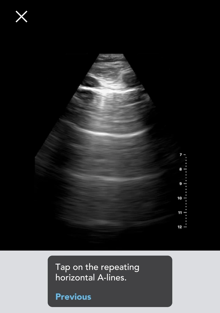
The ACEP SonoGuide includes clinical figures and video examples of several of these artifacts. Static definitions are useful, but recognition improves when you compare the artifact with its cause and observe what happens as the probe moves.

10. Doppler estimates motion from frequency shift

When ultrasound reflects from moving red blood cells, the returning frequency differs from the transmitted frequency. The Doppler shift depends on the transmitted frequency, blood velocity, propagation speed, and the angle between the beam and flow. The angular relationship is critical: as the beam approaches 90 degrees to flow, the measured shift approaches zero even when blood is moving.

Mode	What it displays	Important limitation
Color Doppler	A color map of mean Doppler shifts within a selected box	Color indicates direction relative to the transducer according to the displayed map—not artery versus vein
Power Doppler	Strength of the Doppler signal	Typically does not provide direction or a velocity waveform and is sensitive to motion artifact
Pulsed-wave Doppler	A velocity-versus-time spectrum from a selected sample location	Angle dependent and subject to aliasing when the sampled shift exceeds the scale’s limit
Continuous-wave Doppler	High velocity shifts along the beam	Does not identify the specific depth producing the signal and may not be available on every POCUS system

Aliasing is a display limitation of sampled Doppler, not proof of turbulent flow by itself. Before interpreting a color change or wrapped spectral waveform, check the color map, velocity scale or pulse-repetition frequency, baseline, sample location, gain, and angle. Doppler measurements require application-specific training and should not be reduced to a single color rule.

Doppler angle changes the measured frequency shift. At approximately 90 degrees, the useful Doppler shift approaches zero even when flow is present. Pulsed-wave aliasing is a sampling limitation; changing the baseline alone does not raise the Nyquist limit.

Ultrasound safety: apply ALARA thoughtfully

Diagnostic ultrasound does not use ionizing radiation, but it does introduce acoustic energy into tissue. The U.S. Food and Drug Administration notes that ultrasound can produce mechanical effects and temperature rise in laboratory settings and recommends minimizing exposure while maintaining diagnostic quality.

The American Institute of Ultrasound in Medicine states that no independently confirmed adverse effects from current diagnostic instruments have been reported in human patients in the absence of contrast agents, while also recognizing that greater output and longer exposure can increase the likelihood of bioeffects. AIUM recommends qualified use for medical benefit and exposures that are as low as reasonably achievable.

ALARA means using the lowest acoustic output and shortest scanning time that still obtains the necessary diagnostic information. It does not mean accepting an inadequate examination. Practical habits include:

• Begin with an appropriate application preset and transducer.
• Improve contact, positioning, depth, focus, and receiver gain before increasing output power.
• Monitor the displayed Thermal Index (TI) and Mechanical Index (MI) and understand their application-specific significance.
• Limit dwell time and stop transmitting when active scanning is no longer needed.
• Use Doppler and other higher-output modes only when they add necessary information.
• Follow device instructions, institutional policy, and population-specific professional guidance.

AIUM’s dedicated ALARA statement specifically advises monitoring TI and MI.

A 60-second image optimization checklist

1. Question: State the focused clinical question before touching the controls.
2. Probe and preset: Match the target depth, footprint, and examination type.
3. Contact and position: Add gel, stabilize your hand, and find a workable acoustic window.
4. Orientation: Confirm the probe marker and screen marker relationship.
5. Depth: Show the target with essential anatomy just beyond it.
6. Gain and TGC: Balance brightness without washing out borders or filling fluid with noise.
7. Focus: Place the focal zone at or just deeper than the target.
8. Angle: Make small movements and observe one change at a time.
9. Confirmation: Scan through the structure and obtain another plane or window when appropriate.
10. Safety: Keep output and exposure only as high and long as necessary for the task.

Next, connect these principles to a repeatable practice plan in 10 POCUS tips for beginners. If the broader clinical framework is new, start with what POCUS is and how it differs from comprehensive imaging.

For book-length study, compare our ultrasound physics and SPI book recommendations before choosing a reference or exam-prep companion.

Frequently asked questions

Does ultrasound expose the patient to radiation?

Ultrasound uses non-ionizing sound waves, not the ionizing radiation used by X-ray or CT. It still transmits acoustic energy, which is why qualified operators apply ALARA, monitor output indices, and limit exposure to what is needed for the medical task.

Why does higher frequency improve resolution but reduce depth?

Higher frequency produces a shorter wavelength, which can improve the ability to distinguish small structures. Higher-frequency energy is also attenuated more rapidly in tissue, so less useful signal may return from deep targets.

Is gain the same as output power?

No. Gain amplifies received electronic signals and changes display brightness. Output power changes the acoustic energy transmitted into the patient. Correct the window, depth, focus, and receive gain before increasing output.

Does anechoic always mean simple fluid?

No. Anechoic means few or no echoes were detected. Simple fluid commonly appears anechoic, but settings, angle, artifact, slow flow, and the contents of a collection can change its appearance. Confirm location, shape, posterior features, behavior in another plane, and the clinical context.

Are ultrasound artifacts always errors?

No. An artifact is a consequence of how sound interacted with tissue and how the scanner processed the echoes. Shadowing and posterior enhancement can help characterize a structure, while mirror image or refraction may imitate anatomy. The skill is recognizing the mechanism and testing the finding.

Why can a structure disappear when I tilt the probe?

A smooth or anisotropic structure may return strong echoes only at a narrow range of insonation angles. Tilting can direct the reflected energy away from the transducer. Make a small angle correction and compare the structure in another plane before deciding the change is pathologic.

Can reading ultrasound physics make me competent to scan patients?

No. Physics supports probe selection, image optimization, and artifact recognition, but competence also requires supervised image acquisition, interpretation, integration with clinical context, feedback, quality assurance, and any credentialing required for your role. See how POCUS simulation training fits between hands-on sessions, then find supervised options in the ultrasound events directory.

Turn physics into deliberate practice

Practice these comparisons on an ultrasound phantom, a simulator, or a consenting volunteer or model within a supervised education program. Compare two frequencies on the same target. Move the focus. Reduce unnecessary depth. Change the angle of an anisotropic structure. Follow a shadow to its source. Adjust color scale and observe aliasing. During a clinical examination, change settings only when medically indicated to obtain the necessary information, and follow ALARA rather than experimenting for curiosity. A controlled educational exercise with immediate feedback makes the physics memorable because it explains a visible change.

For off-patient cognitive rehearsal, POCUS Simulator can help you review probe choice, protocol sequence, image interpretation, and clinical cases before supervised scanning. If physical probe mechanics are the missing skill, compare the capabilities of mobile, tracked-probe, and high-fidelity ultrasound simulator formats. Commercial disclosure: POCUS Simulator is an Ultrasound Fanatic product and may include optional in-app purchases. It does not reproduce hands-on probe mechanics or establish competence.

For a quick recall check, open SonoMatch in the browser preview and match probe types and echo appearances to their images. Return to the explanations above for the meaning and limits of each term.

Educational-use disclaimer: This article is a general educational overview, not medical advice, a scanning protocol, or a substitute for device-specific training and supervised clinical education. Perform and interpret ultrasound only within your professional scope, institutional policy, competency, and applicable credentialing requirements.